Accelerated Depreciation

---

1. Accelerated Depreciation

Accelerated depreciation should be used if we have assets that are used more heavily in their earlier years. These are assets that contribute more to production during their earlier years, and lose their functionality over time.

EXAMPLE

Vehicles, for example, are more heavily used in their earlier years. As the wear and tear starts to catch up with a vehicle, it loses its functionality over time.

A main benefit of accelerated depreciation is that there is a reduced time period for writing off that asset's cost, which helps to reduce taxes. This is due to the fact that In the earlier years of that asset's life, you're recording a higher level of depreciation, a greater expense, which will help reduce your taxes.

There are several methods of accelerated depreciation:

• MACRS and ACRS
• Sum of the year's digits
• Units of production
• Double declining balance

1a. MACRS and ACRS

MACRS stands for Modified Accelerated Cost Recovery System, and ACRS is Accelerated Cost Recovery System. These are used when reporting information to the IRS, so when doing your taxes, you need to use MACRS and ACRS as your depreciation method.

1b. Sum of the Year's Digits

Let's take a look at the formula to calculate depreciation using sum of the year's digits. We take the remaining life of the asset as of the beginning of the year and divide it by the sum of the years of the useful life.

formula

Sum of the Year's Digits

This means that if we have an asset with a five-year useful life, our denominator is going to be 5 + 4 + 3 + 2 + 1, or 15. This is how we would set up the calculation for sum of the year's digits--and where it gets its name.

1c. Units of Production

Another method, units of production, is beneficial for machinery. If you have machinery that is used in your production process, it might have a useful life expressed in hours. This could be the number of hours it can be in the production process or the number of units that it can produce.

The formula for units of production takes our depreciable base and multiplies it by the hours this year--the hours that the asset was used during the year--and divides it by the total estimated hours for that asset.

formula

Units of Production

Note, this formula can also be used for units. In this case, you would take the depreciable base, multiply it by units this year, and divide it by total estimated units.

1d. Double Declining Balance

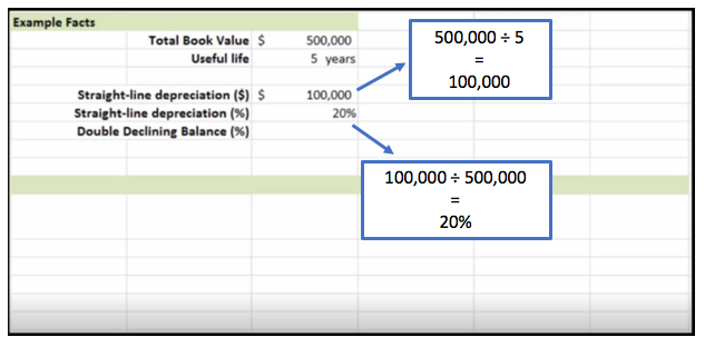
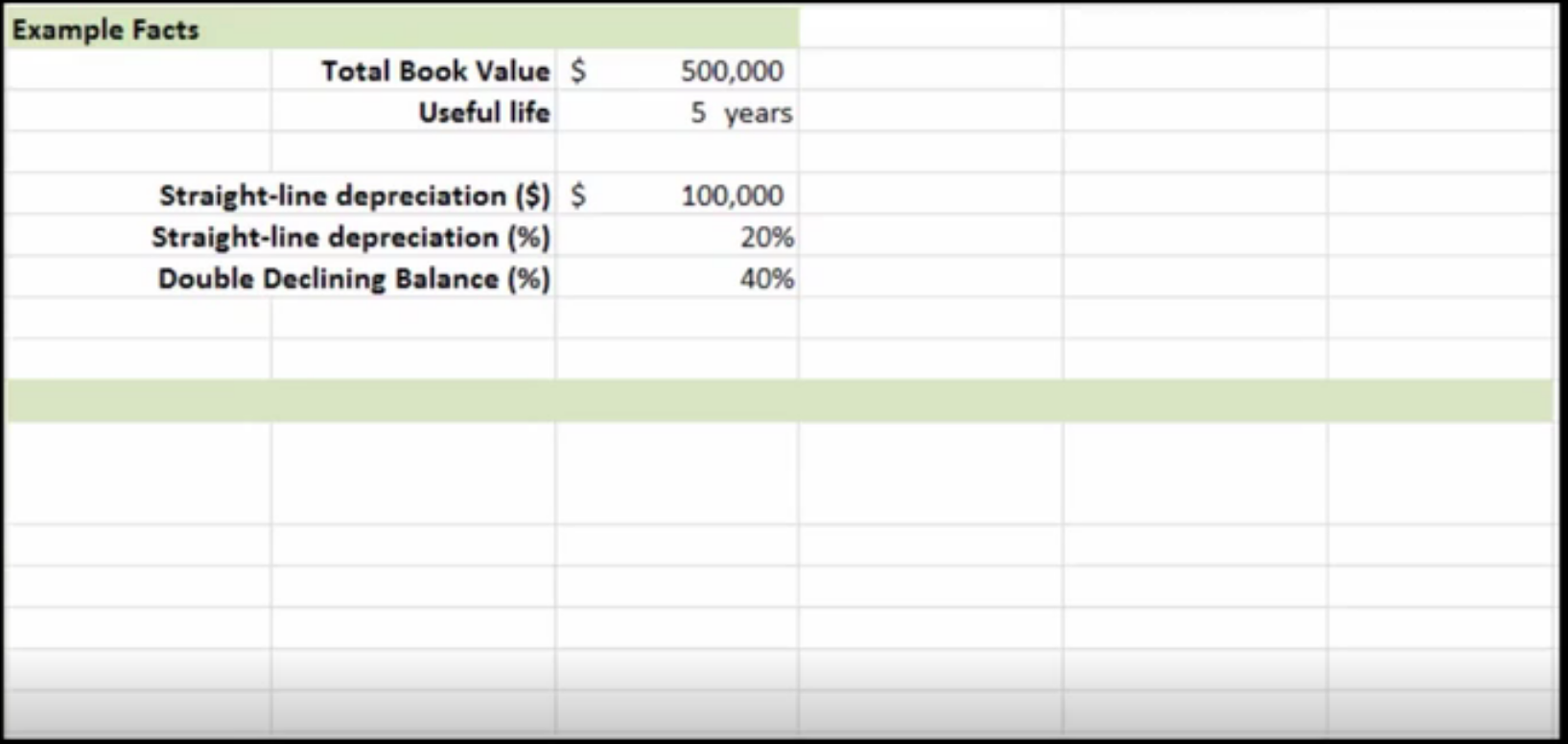
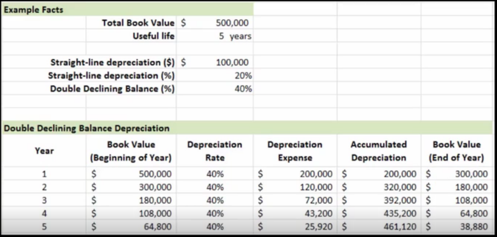
Last, but certainly not least, is double declining balance, which is the most common accelerated depreciation method. One interesting thing about the double declining balance method is that it does not deduct the salvage value when computing the depreciable base.

---

2. Double Declining Balance Example

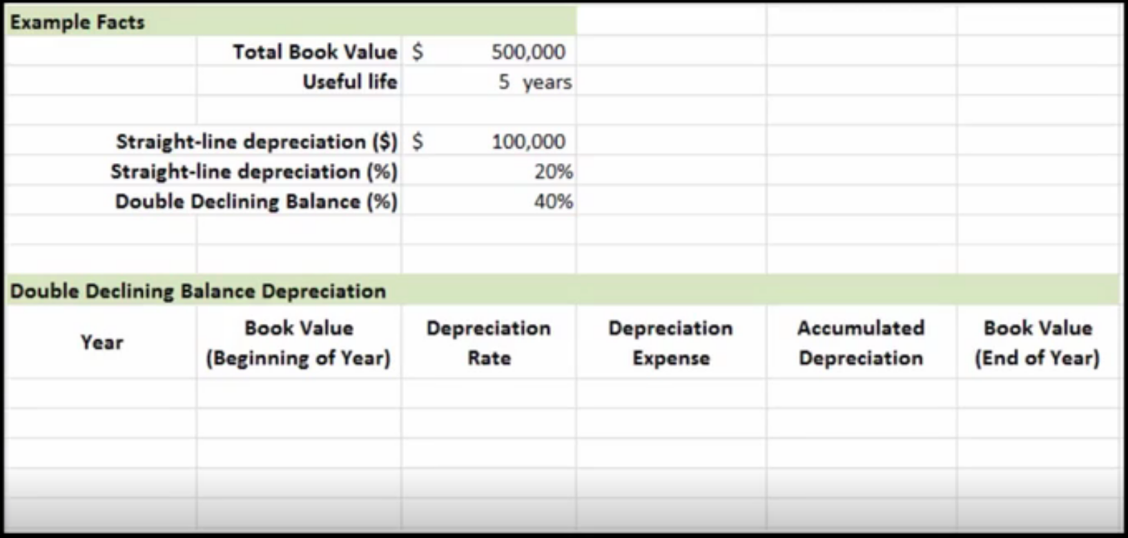
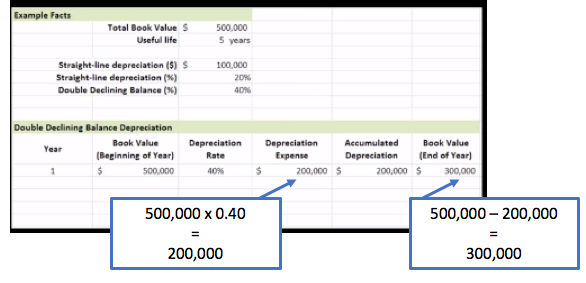
To further explain double declining balance, let's look at an example of calculating depreciation using the double declining balance method.

Step 1
The first step is to determine the straight line rate of depreciation for the year. In this case, we're going to take an asset with a total book value of $500,000 and a useful life of five years.

Now, our straight line depreciation would be $100,000 per year, which is $500,000 divided by 5. We need to express that as a straight line depreciation percentage, which is 20% each year.

Step 2
The next step is to multiply that straight line depreciation rate by 2, which gives us our double declining balance rate.

Step 3
Now that we have the rate for our double declining balance, we can start preparing our depreciation schedule.

The depreciation schedule contain the following columns:

• Year
• Book value at the beginning of the year
• Depreciation rate
• Depreciation expense
• Accumulated depreciation
• Book value at the end of the year

Step 4
The fourth step is to take that double declining balance depreciation rate of 40% and apply it to our asset, in the "Depreciation Rate" column.

We apply it to the initial value, and in the subsequent years, we apply that double declining balance rate to the carrying value at the beginning of the year.

As you can see at the beginning of the year in year two, our book value is the same book value that we ended the first year with.

We would complete this process for all five years. You can see that at the end of year five, we have a book value of $38,880.

---

3. Depreciation Calculation Comparison

We have one final visual representation to examine. Here we have the same example facts as before, only now we've added production life for our units of production method, as well as the production hours over the course of the life of this example asset.

We're going to look at the comparison of these three depreciation methods--double declining balance, sum of the year's digits, and units of production.

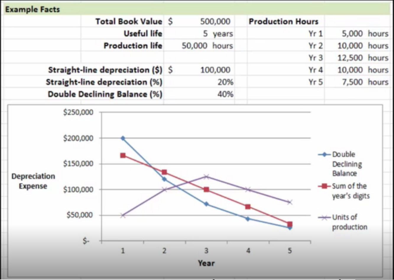
You'll see with that double declining balance, in the early years the depreciation is greater and then starts to taper off towards the end of that asset's useful life.

In sum of the year's digits, it's a very linear, downward sloping line, because it's systematically decreasing over time.

Lastly, units of production is based entirely on the amount of production, so the trajectory of depreciation depends on the production over time. There might be spikes in depreciation, and then as that asset starts to age, its productivity decreases.

---