Table of Contents |
In the last lesson, you learned about how a single extreme value, or outlier, can have an outsized effect on measuring data variability with range. Consequently, the range is not always a reliable measure of the variability in your data. In this lesson, you will learn about a better way to measure the spread of your data.
The range is an important summary of variability in your data. However, often we are interested in making comparisons to other observations. Splitting your information into groups called quartiles, which each represent 25% of the data, is useful for these comparisons.
A weakness of the standard range calculation is that it can be thrown off by a single extreme value, causing the range to be a poor representation of the true variability. For instance, having just one very tall or very short individual can affect the range of a data set consisting of thousands of individuals. In a case such as this, it’s useful to have a measure of variability that more accurately captures the overall data variability. Such a measure of variability is known as the interquartile range (IQR).
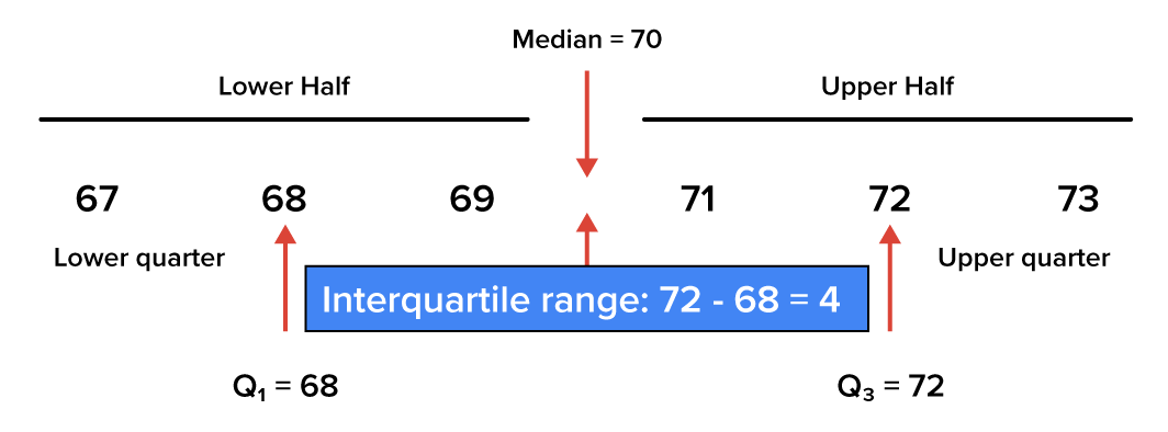
A chart of men’s heights will have a normal distribution. The median height for men, as shown below, is roughly 70 inches. The quartiles are broken down here:
1st Quartile: < 68 inches
2nd Quartile: 68-70 inches
3rd Quartile: 70-72 inches
4th Quartile: > 72 inches

According to this, anything less than 68 inches will be in the first quartile, anything between 68 and 70 inches will be in the second quartile, between 70 and 72 in the third, and anything above 72 inches will be in the fourth quartile.
While the range represents the entire extent of the data set, the interquartile range represents the middle 50% of the data set. Like the range, the interquartile range is a measure of variability or spread. The larger the interquartile range, the more spread out the values in the middle 50% of the data set are. The interquartile range is a more reliable measure of the spread of data than the standard range because it takes into account all data, not only the maximum and minimum values.
To find the interquartile range of a data set, find the first quartile (Q₁) and the third quartile (Q₃). The interquartile range, then, is the difference between the third quartile and the first quartile. To consider the middle portion of the data, you are only concerned about the first and the third quartiles.
So, how do we go about figuring this out?
First, sort the data from smallest to largest value, and then divide it into two halves. The middle value would be the median. Next, find the middle value of the first half. This is the first quartile, Q₁. Third, determine the middle value of the second half. This would be the third quartile, or Q₃.
Let’s look at a hypothetical data set that involves the income of 25- to 34-year-olds:
| $20,000 | $57,000 |
| $27,000 | $61,000 |
| $29,000 | $62,000 |
| $32,000 | $66,000 |
| $33,000 | $71,000 |
| $36,000 | $77,000 |
| $40,000 | $84,000 |
| $43,000 | $88,000 |
| $45,000 | $96,000 |
| $48,000 | $102,000 |
| $50,000 | $107,000 |
Use the above information to calculate the interquartile range.
Establish the midpoint, then find the middle value of the first half and the middle value of the second half.
The midpoint for all the data is between the values of $50,000 and $57,000, which comes out to be $53,500.
Midpoint = Median = $53,500 (Q₂)
The middle of the first half of the numbers is the middle value of the first 11 numbers, or $36,000.
Q₁ = $36,000
The middle of the second half of the numbers is the middle value of the second 11 numbers, or $77,000.
Q₃ = $77,000
Now take $77,000 minus $36,000 to get $41,000. That is the interquartile range for this group of income.
Notice how that compares to the range, which is $87,000 ($107,000 - $20,000). That is twice as much as the interquartile range. You can see how the interquartile range gives us a much better measure of variability.
Source: THIS TUTORIAL WAS AUTHORED BY DAN LAUB FOR SOPHIA LEARNING. PLEASE SEE OUR TERMS OF USE.