Confidence Intervals Using the T-Distribution

1. Confidence Interval Using the T-Distribution

A confidence interval using the t-distribution is very similar to a hypothesis test. In fact, it is preferred to a hypothesis test because we have an estimate and a conclusion that can be made equivalent to a two-tailed test.

When calculating the confidence interval for a sampling distribution, you would normally take the sample mean plus or minus some number of standard deviations times the standard error, or .

However, the only problem is this formula has a sigma in it, which is the population standard deviation. For situations where we don't know what the population standard deviation is, you have to replace this formula with one that uses "s", or the sample standard deviation.

Since you're using s as a stand-in for sigma, you need to use the t-distribution instead and come up with the following formula:

formula to know

Confidence Interval of Population Mean

terms to know

Confidence Interval

An interval we are some percent certain (eg 90%, 95%, or 99%) will contain the population parameter, given the value of our sample statistic.

T-Distribution

A distribution similar to the normal distribution but with fatter tails. Depending on the sample size, it does not diminish toward the tails as fast.

2. Constructing a Confidence Interval Using the T-Distribution

To construct a confidence interval for population means using the t-distribution, the following steps must be followed:

step by step

Step 1: Verify the conditions necessary for inference.
Step 2: Calculate the confidence interval.
Step 3: Interpret the confidence interval.

EXAMPLE

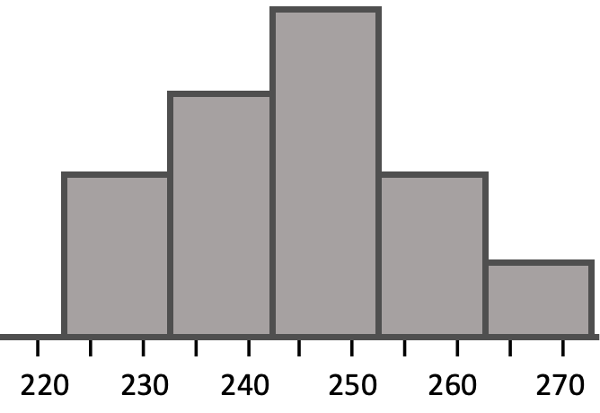
Many times, consumers will pay attention to nutritional contents on packaged food so it's important to make them accurate as to what the food product actually contains. Suppose, for example, that the stated calorie content for a particular frozen dinner was 240.

A random sample of 12 frozen dinners was selected, and the calorie contents of each one was determined.

255	244	239	242	265	245
259	248	225	226	251	233

One of the boxes actually contained 255 calories worth of food whereas another one only contained 225 calories' worth of food. We can quickly calculate the mean and standard deviation by using Excel.

First, enter all 12 values. Go to the Formulas tab, and we will use the formula AVERAGE under the Statistical option to find the sample mean and highlight all the values.


The sample mean is 244.33 calories. To find the sample standard deviation, again go under the Formulas tab, and select STDEV.S under the Statistical option. Highlight all 12 values.


The sample standard deviation is 12.38.

Suppose you want to construct a 90% confidence interval for the true mean number of calories. This means that you want to construct a confidence interval such that you’re 90% confident that the true mean of all the packaged frozen dinners lies within the interval.

Step 1: Verify the conditions for inference.

Stating the conditions isn't enough, and it's not just a formality--you must verify them. Recall the conditions needed:

Condition	Description
Randomness	How was the sample obtained?
Independence	Population ≥ 10n
Normality	n ≥ 30 or normal parent distribution

Let's go back to our example to check the requirements of randomness, independence, and normality.

• Randomness: It was a random sample, as was said in the problem.
• Independence: Is the population of all frozen dinners at least 10 times the size of your sample? That's reasonable to believe. Assume there are at least 120 frozen dinners in all of this company's frozen dinner line.
• Normality: This one's a little tricky. Your sample size isn't 30 or larger, so the Central Limit Theorem doesn't apply to this problem. Is the parent distribution normal? You don't know that either. You need to determine if this is plausible. You can do that by graphing the actual data that you have.

You can see that the parent distribution might be normal since the data that you got from the population are single peaked and approximately symmetric. It's possible that the population parent distribution is normal. You can proceed under the assumption of normality. You can’t verify it 100%, but assume it is for the purposes of this problem.

Step 2: Calculate the confidence interval.

Reviewing the formula, we need the sample mean, the sample standard deviation, the sample size, and the t-critical value. We have already figured out the information about the sample with the help from Excel:



We know that 244.33 is the sample mean and the standard deviation is 12.38 when we used the data of the 12 dinners. This information also tells us that the sample size is 12. What we still need to do is figure out what that t* value is going to be.

To find this value, we need a t-distribution table. We need a t* that will give us 90% of the t-distribution. 90% confidence interval would mean that there is 10% remaining on either side for the two tails, or 5% for each tail.

Looking at the table, we can match this information with the values 0.05 in the row of one-tailed or 0.10 in the row of two-tailed. We can also look all the way down at the bottom and see that there is a row that says "Confidence Interval." There is 50%, 60%, 70%, 80%, 90%, etc. Either one of those justifications is reason enough to use this column.

We also need to know the degrees of freedom to determine which number from this column we're going to use. In this problem, we have 11 degrees of freedom because we had 12 dinners in our sample, and the degrees of freedom is n minus 1.



So we need to look for the corresponding value inside that table that matches with 11 degrees of freedom and 90% confidence interval.

t-Distribution Critical Values
Tail Probability, p
One-tail	0.25	0.20	0.15	0.10	0.05	0.025	0.02	0.01	0.005	0.0025	0.001	0.0005
Two-tail	0.50	0.40	0.30	0.20	0.10	0.05	0.04	0.02	0.01	0.005	0.002	0.001
df
1	1.000	1.376	1.963	3.078	6.314	12.71	15.89	31.82	63.66	127.3	318.3	636.6
2	0.816	1.080	1.386	1.886	2.920	4.303	4.849	6.965	9.925	14.09	22.33	31.60
3	0.765	0.978	1.250	1.638	2.353	3.182	3.482	4.541	5.841	7.453	10.21	12.92
4	0.741	0.941	1.190	1.533	2.132	2.776	2.999	3.747	4.604	5.598	7.173	8.610
5	0.727	0.920	1.156	1.476	2.015	2.571	2.757	3.365	4.032	4.773	5.893	6.869
6	0.718	0.906	1.134	1.440	1.943	2.447	2.612	3.143	3.707	4.317	5.208	5.959
7	0.711	0.896	1.119	1.415	1.895	2.365	2.517	2.998	3.499	4.029	4.785	5.408
8	0.706	0.889	1.108	1.397	1.860	2.306	2.449	2.896	3.355	3.833	4.501	5.041
9	0.703	0.883	1.100	1.383	1.833	2.262	2.398	2.821	3.250	3.690	4.297	4.781
10	0.700	0.879	1.093	1.372	1.812	2.228	2.359	2.764	3.169	3.581	4.144	4.587
11	0.697	0.876	1.088	1.363	1.796	2.201	2.328	2.718	3.106	3.497	4.025	4.437
12	0.695	0.873	1.083	1.356	1.782	2.179	2.303	2.681	3.055	3.428	3.930	4.318
13	0.694	0.870	1.079	1.350	1.771	2.160	2.282	2.650	3.012	3.372	3.852	4.221
14	0.692	0.868	1.076	1.345	1.761	2.145	2.264	2.624	2.977	3.326	3.787	4.140
15	0.691	0.866	1.074	1.341	1.753	2.131	2.249	2.602	2.947	3.286	3.733	4.073
16	0.690	0.865	1.071	1.337	1.746	2.120	2.235	2.583	2.921	3.252	3.686	4.015
17	0.689	0.863	1.069	1.333	1.740	2.110	2.224	2.567	2.898	3.222	3.646	3.965
18	0.688	0.862	1.067	1.330	1.734	2.101	2.214	2.552	2.878	3.197	3.610	3.922
19	0.688	0.861	1.066	1.328	1.729	2.093	2.205	2.539	2.861	3.174	3.579	3.883
20	0.687	0.860	1.064	1.325	1.725	2.086	2.197	2.528	2.845	3.153	3.552	3.850
21	0.686	0.859	1.063	1.323	1.721	2.080	2.189	2.518	2.831	3.135	3.527	3.819
22	0.686	0.858	1.061	1.321	1.717	2.074	2.183	2.508	2.819	3.119	3.505	3.792
23	0.685	0.858	1.060	1.319	1.714	2.069	2.177	2.500	2.807	3.104	3.485	3.767
24	0.685	0.857	1.059	1.318	1.711	2.064	2.172	2.492	2.797	3.091	3.467	3.745
25	0.684	0.856	1.058	1.316	1.708	2.060	2.167	2.485	2.787	3.078	3.450	3.725
26	0.684	0.856	1.058	1.315	1.706	2.056	2.162	2.479	2.779	3.067	3.435	3.707
27	0.684	0.855	1.057	1.314	1.703	2.052	2.158	2.473	2.771	3.057	3.421	3.690
28	0.683	0.855	1.056	1.313	1.701	2.048	2.154	2.467	2.763	3.047	3.408	3.674
29	0.683	0.854	1.055	1.311	1.699	2.045	2.150	2.462	2.756	3.038	3.396	3.659
30	0.683	0.854	1.055	1.310	1.697	2.042	2.147	2.457	2.750	3.030	3.385	3.646
40	0.681	0.851	1.050	1.303	1.684	2.021	2.123	2.423	2.704	2.971	3.307	3.551
50	0.679	0.849	1.047	1.299	1.676	2.009	2.109	2.403	2.678	2.937	3.261	3.496
60	0.679	0.848	1.045	1.296	1.671	2.000	2.099	2.390	2.660	2.915	3.232	3.460
80	0.678	0.846	1.043	1.292	1.664	1.990	2.088	2.374	2.639	2.887	3.195	3.416
100	0.677	0.845	1.042	1.290	1.660	1.984	2.081	2.364	2.626	2.871	3.174	3.390
1000	0.675	0.842	1.037	1.282	1.646	1.962	2.056	2.330	2.581	2.813	3.098	3.300
>1000	0.674	0.841	1.036	1.282	1.645	1.960	2.054	2.326	2.576	2.807	3.091	3.291
	Confidence Interval between -t and t
	50%	60%	70%	80%	90%	95%	96%	98%	99%	99.5%	99.8%	99.9%

Look in the 11 degrees of freedom row and the 90% confidence column until we obtain a t* of 1.796.

Now we have all the information needed in order to create our confidence interval. Construct it as x-bar plus or minus the t critical value times the sample standard deviation divided by the square root of sample size.



When we do that, we obtain 244.33 plus or minus 6.42. When we evaluate the interval, it's going to be 237.68 all the way up to 249.98.



Step 3: Interpret the confidence interval.

What does this confidence interval actually mean? How can you interpret the interval? The interpretation is that we're 90% confident that the true mean calorie content of all frozen dinners is between about 237 and 250 calories. We're 90% confident that the real value is somewhere in there, and that the 240 value that they were purporting at the beginning of the problem is, in fact, plausible.