Use Sophia to knock out your gen-ed requirements quickly and affordably. Learn more
×

Distribution of Sample Means

Author: Sophia

what's covered
This tutorial will cover the distribution of sample means. Our discussion breaks down as follows:

Table of Contents

1. Distribution of Sample Means

A distribution of sample means is a distribution that shows the means from all possible samples of a given size.

EXAMPLE

Consider the spinner shown here:
Spinner
Suppose you spun it four times to obtain a sample mean. The first spin was a 2, the second spin was a 4, the third spin was a 3, and the fourth spin was a 1. The sample mean, then, would be 2.50. There's are many possible samples that could be taken of size 4 for this spinner, and there are many possible means that could arise from those samples, as shown below:

Sample Mean
S subscript 1 = {2, 4, 3, 1} x with bar on top subscript 1 = 2.50
S subscript 2 = {1, 4, 3, 1} x with bar on top subscript 2 = 2.25
S subscript 3 = {4, 2, 4, 4} x with bar on top subscript 3 = 3.50
S subscript 4 = {2, 2, 3, 1} x with bar on top subscript 4 = 2.00
S subscript 5 = {3, 1, 1, 1} x with bar on top subscript 5 = 1.50
S subscript 6 = {1, 1, 1, 2} x with bar on top subscript 6 = 1.25

So how can we represent all these distributions?

step by step
Step 1: First, take these sample means and graph them. Draw out an axis. For this one, it should go from 1 to 4 because this set can’t average anything higher than four or lower than a one.

Step 2: Take the average value, for example, the mean of 2.5, and put a dot at 2.5 on the x-axis, much like a dot plot. Do this for all the sample means that you have found. Distribution of the first six samples

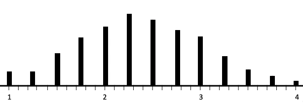
Step 3: You can keep doing this over and over again. Ideally, you would do this hundreds or thousands of times, to show the distribution of all possible samples that could be taken of size four. Once you’ve enumerated every possible sample of size four from this spinner, then the sampling distribution looks like this:

Sampling Distribution

On the graph, the lowest number you can get is one, and the highest number you can get is four. On the far right of the graph is the point that represents a spin of 4 fours, {4, 4, 4, 4}. On the far left is the point that represents a spin of 4 ones, {1, 1, 1, 1}. Notice that 4 ones happens more than 4 fours. Why is that? If you take a look at the spinner, you'll see that there are more ones on the spinner than there are fours.

You can also notice that, since there are more ones, this actually pulls the average down a bit. The most frequent average is 2.25, not 2.5, which would be the exact middle between 1 and 4. Therefore, this distribution is skewed slightly to the right because the numbers on the spinner are not evenly distributed.

term to know
Distribution of Sample Means
A distribution where each data point consists of a mean of a collected sample. For a given sample size, every possible sample mean will be plotted in the distribution.

1a. Mean

EXAMPLE

For the spinner above, the following are the histograms for a sample size of 1 spin, 4 spins, 9 spins, and 20 spins.
Sampling Distribution for Sample Size One
Sampling Distribution for Sample Size Four
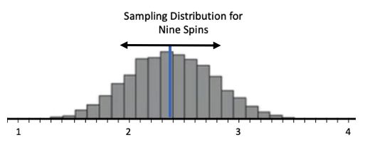
Sampling Distribution for Sample Size Nine
Sampling Distribution for Sample Size 20

With the sampling distribution when the sample size was 1, you'll see that 1 occurs about 3/8 of the time, 2 occurs about 1/8 of the time, 3 occurs about a fourth of the time, and 4 occurs about a fourth of the time. This produces a mean of 2.375:

m e a n equals fraction numerator 1 plus 1 plus 1 plus 2 plus 3 plus 3 plus 4 plus 4 over denominator 8 end fraction equals 19 over 8 equals 2.375

You'll notice that when the sample size is 4, the shape of the distribution of sample means is significantly different from when the sample size was 1. However, there some similarities and differences that you can recognize here about all four of these sampling distributions. The similarities are their centers--all of them are centered at 2.375. You'll notice that some of these are more tightly packed around that number--for instance, the samples of size 20 are more tightly packed around 2.375 than the samples of size 1--but they all are centered at that very same number.
Sampling Distribution for Sample Size One
Sampling Distribution for Sample Size Four
Sampling Distribution for Sample Size Nine
Sampling Distribution for Sample Size 20

What we can see here is that the mean of the sampling distribution of sample means is the same as the mean for the population. In this case, it was 2.375.

formula to know
Mean of a Sampling Distribution of Sample Means
mu subscript x with bar on top end subscript equals mu subscript p o p u l a t i o n end subscript

1b. Standard Deviation

EXAMPLE

How about the spread? The arrows on each of the histograms below indicate the standard deviation of each distribution.
Standard Deviation of Sample Distribution for Sample Size One
Standard Deviation of Sample Distribution for Sample Size Four
Standard Deviation of Sample Distribution for Sample Size Nine
Standard Deviation of Sample Distribution for Sample Size 20

Notice the arrows on the first distribution are very wide, and they seem to diminish in size as each distribution is graphed. When we get to the lowest distribution where the sample size was 20, its spread is much, much less.

The rule that's being followed is that the standard deviation of a distribution of sample means is the standard deviation of the population divided by the square root of sample size.

formula to know
Standard Deviation of a Sampling Distribution of Sample Means
sigma subscript x with bar on top end subscript equals fraction numerator sigma subscript p o p u l a t i o n end subscript over denominator square root of n end fraction

What that indicates is that when the sample size is 4, the standard deviation of that sampling distribution of sample means is going to be half as large as it was when the sample size was one. When the sample size is 9, it's going to be a third the size of the original standard deviation. And when n is 20, it's going to be the original standard deviation divided by the square root of 20.

hint
The standard deviation of the sampling distribution is also called the standard error.

terms to know
Standard Deviation of a Distribution of Sample Means
The standard deviation of the population, divided by the square root of sample size.
Standard Error
The standard deviation of the sampling distribution of sample means.

1c. Shape

EXAMPLE

Lastly, let's discuss the measured center, or measured spread, and describe the shape of these distributions. You'll notice that the shape is becoming more and more like the normal distribution as the sample size increases. There's a theorem that describes that, called the central limit theorem.

The Central Limit Theorem states that when the sample size is large (at least 30 for most distributions with a finite standard deviation), the sampling distribution of the sample means is approximately normal.

This means we can use the normal distribution to calculate probabilities on them, which is nice because normal calculations are easy to do.

Therefore, it's going to be normal, or approximately normal, with a mean of the same as that of the population, and a standard deviation equal to the standard deviation of the population divided by the square root of sample size.

term to know
Central Limit Theorem
A theorem that explains the shape of a sampling distribution of sample means. It states that if the sample size is large (generally n ≥ 30), and the standard deviation of the population is finite, then the distribution of sample means will be approximately normal.

summary
The distribution of sample means is called a sampling distribution of sample means. The sampling distribution of sample means has an approximately normal sampling distribution when the sample size is large. This is the Central Limit Theorem. The mean of the sampling distribution is the mean of the population. The standard deviation of the sampling distribution, which is also called the standard error, is the standard deviation of the population divided by the square root of the sample size.

Good luck!

Source: THIS TUTORIAL WAS AUTHORED BY JONATHAN OSTERS FOR SOPHIA LEARNING. PLEASE SEE OUR TERMS OF USE.

Terms to Know
Central Limit Theorem

A theorem that explains the shape of a sampling distribution of sample means. It states that if the sample size is large (generally n ≥ 30), and the standard deviation of the population is finite, then the distribution of sample means will be approximately normal.

Distribution of Sample Means

A distribution where each data point consists of a mean of a collected sample. For a given sample size, every possible sample mean will be plotted in the distribution.

Standard Deviation of a Distribution of Sample Means

The standard deviation of the population, divided by the square root of sample size.

Standard Error

The standard deviation of the sampling distribution of sample means distribution.

Formulas to Know
Mean of a Sampling Distribution of Sample Means

mu subscript x with bar on top end subscript space equals space mu subscript p o p u l a t i o n end subscript

Standard Deviation of a Sampling Distribution of Sample Means

sigma subscript x with bar on top end subscript space equals space fraction numerator sigma subscript p o p u l a t i o n end subscript over denominator square root of n end fraction