Common sense tells us that when we make more money, we tend to buy more. However, is it the same for all goods?
The idea of elasticity, in general, involves how much we change our minds, or how much more or less we buy as a variable is changing.
Income elasticity is different than own-price or cross-price elasticity, because it refers to our income changing instead of price.
Income elasticity is an economic measure of change in relation to income and demand for normal, inferior, and luxury goods.
Here is the equation, which we were able to simplify down to the percentage change in quantity divided by the percentage change in income.

Let's start by looking at an example using Nike. If our income rises, will we buy more or less Nike apparel?
Suppose Tom's income increases from $20,000 to $40,000. He used to buy two pair of Nike running shoes a year, but now he can afford to buy three pairs.
| Quantity of Nike Shoes | Income |
|---|---|
| QA = 2 Pairs | IA = $20,000 |
| QB = 3 Pairs | IB = $40,000 |
Tom's demand curve is shown below. Notice, though, this demand curve looks different than the normal demand curve that you are used to seeing.
Instead of looking at what happens to demand when the price of an item changes, we are looking at what happens when someone's income changes.
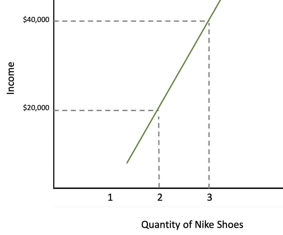
As you can see, there is a positive relationship between Tom's income and Nike shoes purchased.
Let's plug our numbers into the income elasticity equation. We are looking at the percentage change in the quantity of Nike he is buying, divided by the percentage change in his income.

Because both the numerator and denominator are negative, they cancel out, giving us a positive .61.
However, what does this number actually tell us?
Generally speaking, quantity and price are going to move in opposite directions.
EXAMPLE
As the price of Nike goes up, the quantity that people purchase goes down.However, with income elasticity:
Therefore, like in our Nike example, if the coefficient is positive, this tells us that these two variables move in the same direction.
As income rises, we buy more, while as income falls, we buy less.
Most goods are normal goods and behave this way, and Nike, as it turns out in Tom's example, is a normal good.
On the other hand, if the coefficient were to be negative, then the good would be inferior because that would suggest that as income rises--the denominator would be positive--the percentage change in quantity (numerator) would be negative, meaning we would buy less of it.
Conversely, as income falls, we would buy more of an inferior product.
A normal good is defined simply as goods for which demand increases as income increases. Again, these are most goods.
Next, let's look at a special kind of normal good, using the example of a vacation.
Notice that when our income is $40,000, we can't afford to go on any vacations at all. As our income doubles to $80,000, we can go on vacation three times in a year.
| Quantity of Vacations | Income |
|---|---|
| QA = 0 | IA = $40,000 |
| QB = 3 | IB = $80,000 |
So, looking at our income on the y-axis and the quantity on the x-axis, notice that there is a positive relationship between income and vacations purchased, just as there was with Nike shoes.

Therefore, this is going to be a normal good--but it's a special kind of normal good.
Once again, let's plug our numbers into the income elasticity equation.

We get two negatives which cancel out and give us a positive number.
However, our last positive number was a decimal; it was 0.61. This coefficient is a lot larger.
With an elasticity of 3, we are going to classify this as a luxury good.
Coefficients that are greater than 1 indicate that when our income increases by 1%, for example, our purchases of the good increase by more than 1%.
In fact, we weren't able to afford any vacations at all before our income changed and now, all of a sudden, we are able to afford three.
Therefore, this is what is considered a luxury good, which is a good that offers better quality and features, which is consumed when income rises.
EXAMPLE
Other examples of luxury goods are high-end luxury cars and artwork. These are items that you do not purchase any amount of before your income increases.Let's look at our last example, which features a generic cereal.
We will be graphing the quantity on the x-axis and our income, again, on the y-axis.
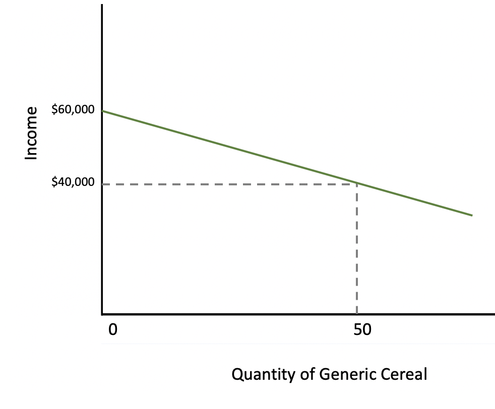
Notice that this curve is downward sloping. This is showing us that when our income is $40,000, we buy 50 boxes of generic cereal a year.
When our income rises to $60,000, we actually don't buy any generic cereal anymore.
There is a negative relationship between our income and the amount of generic cereal we are purchasing.
As we make more money, we stop buying generic products and start to opt for name brands.
Let's use the same formula and keep in mind that the order is going to matter again.

We get a positive numerator and negative denominator, which leaves us with a negative number.
Remember, a negative number tells us that it is an inferior good, because there is a negative relationship between income and our consumption.
As our income rises, we buy less of this type of good. As our income falls, we would buy more.
Therefore, inferior goods are goods for which demand decreases as income increases.
| Income Elasticity Coefficients | |
|---|---|
| E < 0 | Inferior Good |
| E > 0 | Normal Good |
| E > 1 | Luxury Good |
Source: Adapted from Sophia instructor Kate Eskra.
