Introduction to Significance Levels

1. Sampling and Significance Levels

The benefit of taking random samples from a population is that it enables us to get a more representative estimation of what the population actually looks like. When you draw a lot of random samples, the result is having a sample mean for each sample, or a lot of sample means. In the event that the sample sizes are large enough, the sample means will be normally distributed and centered on the mean of the population.

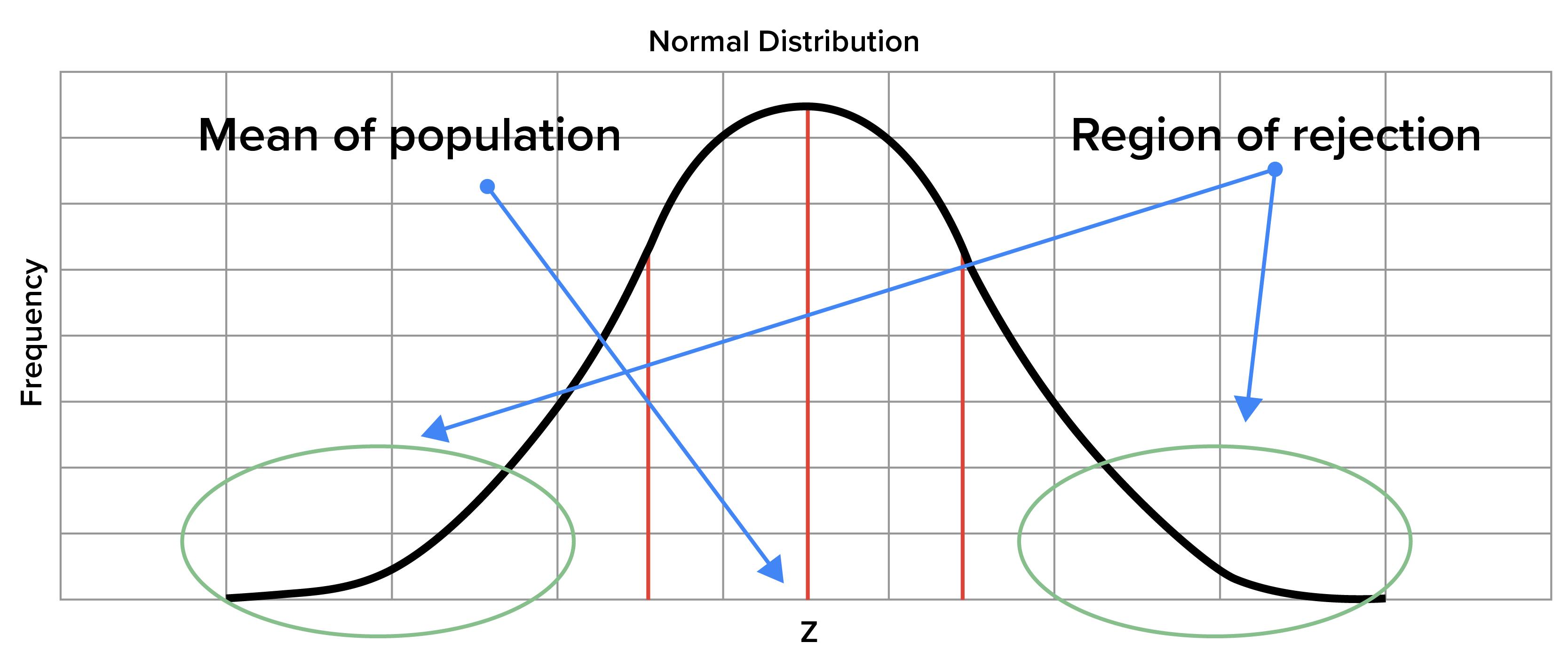
When sampling data, it is helpful to know which sampling means are very large and which are very small. This could be done by selecting a region on a normal distribution that falls far away from the mean in both directions. This area on the distribution is referred to as the region of rejection. It represents that part of the distribution in which the results are not likely to be due to chance.

This area of the region is known as the significance level, a level that is typically chosen to be 5%. Sample means that fall into this region of rejection are generally considered vastly different from the population mean and are unlikely to occur as sample means.

2. Determining a Region of Rejection

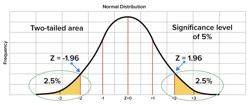
The areas of the region of rejection lie in the areas to the left of z = -1.96 and to the right of z = 1.96. This is what is called a two-tailed area. One tail lies to the far right of the distribution and the other to the far left, with each comprising 2.5% of the total area under the curve. When considering a z-table, these 2.5% areas translate to z-scores of less than - 1.96 and greater than 1.96. This 5% combined area of the region of rejection relates to the significance level of 5%.

try it

Suppose you have an example of a normally distributed variable in which there are four observations that interest you:

• z = 2.81
• z = 1.54
• z = -2.05
• z = -0.46

Which of these z-scores lie in the region of rejection?

The z-score of 2.81 falls to the right of z = 1.96 and the z-score of -2.05 falls to the left of z = -1.96, so both scores are in the region of rejection. However, the z-scores of 1.54, which does not fall to the right of z = 1.96, and -0.46, which does not fall to the left of z = -1.96, do not fall in the region of rejection.

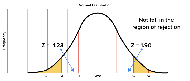
When a z-value lies in the region of rejection, it is understood that the corresponding sample mean varies significantly from the population mean. The z-scores of 1.90 and -1.23 would not fall in the region of rejection, which means that the sample means corresponding to these z-scores would not be rejected, because they do not vary significantly from the population mean.