Solving Systems of Linear Inequalities by Graphing

1. Graphing a Linear Inequality

When graphing a linear inequality, we follow a similar process to graphing a linear equation. In fact, we can first think of the inequality as an equation, with an equals sign rather than an inequality symbol, and graph the line. When we do this, what we are really doing is graphing the boundary line to the inequality. To correctly graph the boundary line, we need to consider whether the inequality symbol is strict or non-strict:

We also need to shade half of the coordinate plane when graphing an inequality, to show which coordinate pairs (x, y) represent solutions to the inequality. When boundary lines are written in the form , the type of inequality symbol tells us to shade either above or below the line:

2. Graphical Solution to a System of Inequalities

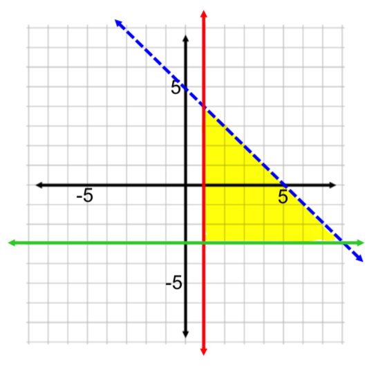
When graphing a system of inequalities, we have more than one inequality graphed on the same coordinate plane. Solution regions to individual inequalities will overlap with other solution regions, but not necessarily all other solution regions. A solution to the entire system of inequalities is the overlap of all of the individual solution regions.

hint

It is important to remember that the solution region to the system is the overlap of all solution regions to each individual inequality in the system. Some areas of the coordinate plane will represent overlap between some of the inequalities, but not all, and would thus not represent a solution to the system.

3. Solving a System of Inequalities by Graphing

Let's solve a system of inequalities using a graphical approach, rather than using algebraic techniques to solve. To do so, we will plot each inequality individually, along with its solution region. Then, we will analyze the graph to determine if there exists an overlap between all solution regions to the inequalities that make up our system.

EXAMPLE

Solve the following system of inequalities by graphing:

We'll start by graphing each of these inequalities one by one, on the same coordinate plane.

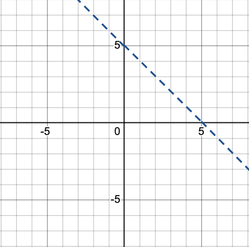
To graph , we take note of the strict inequality symbol, which tells us to use a dashed line to graph the boundary line . This linear equation is in standard form, so we can graph this line by finding the x- and y-intercepts. Alternatively, you could change this into slope-intercept form and graph it that way. Using standard form, when , then , so the x–intercept is the point (5, 0). Similarly, when , then , so the y–intercept is (0, 5). Plot these two points and connect them with a dashed line.



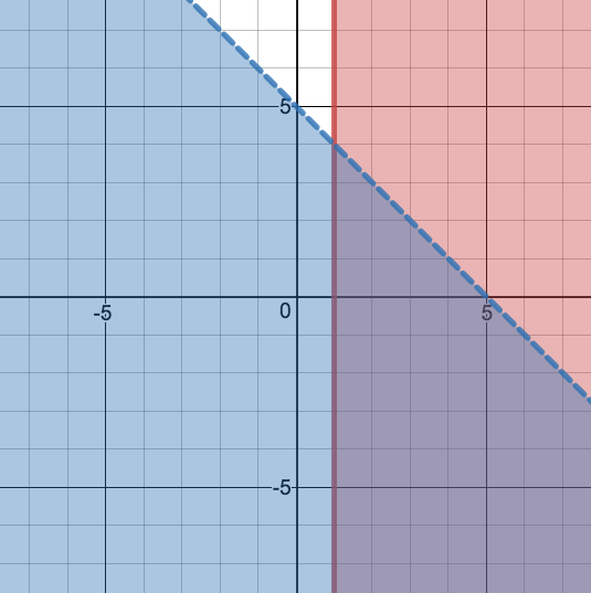
Finally, we need to decide which part of the coordinate plane to shade. But be careful about the general tip to interpret < and ≤ as shading below the line, and interpreting the symbols > and ≥ as shading above the lines! This is only useful when we have y on one side of the equation by itself, and everything else on the other side. With inequalities such as , we should use a test point.

Let's use the test point (0, 0) to plug into our inequality. We substitute 0 in for x and 0 in for y, and see if our statement is true or false. Since is a true statement (because 0 is less than 5), the point (0, 0) lies within the solution region, and we shade the half-plane that includes this point.



Next, we'll add the inequality to our graph. This inequality is quite simple to graph because it is a vertical line. We'll just take note of our inequality symbol to determine what kind of line to draw, and which region to shade. Our inequality symbol is non-strict, so we use a solid line, and we'll shade to the right of the line because that represents greater x-values.



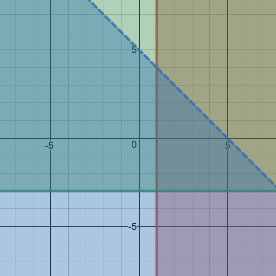
With the final inequality , it is also quite simple to graph as it is a horizontal line. We once again look at the inequality symbol: it is non-strict, so we will use a solid line to draw the boundary line. Since the symbol is "greater than or equal to" we also know to shade above the boundary line.



At this point, it's a bit unclear to see the solution region to the system. The solution region to the system is the overlap between all individual solution regions: